Symbolic Regression on
Network Properties


Marcus Märtens, Fernando Kuipers and Piet Van Mieghem

Follow this presentation on your device: https://coolrunning.github.io/symbreg_pres

NAS logo Network
Architectures and
Services
TU Delft logo

Network representations

  • Number of nodes: $N$
  • Number of links: $L$

Adjacency matrix $A = \begin{bmatrix} 0 & 1 & 1 & 1 & 1 & 0 \\ 1 & 0 & 0 & 0 & 1 & 1 \\ 1 & 0 & 0 & 1 & 1 & 0 \\ 1 & 0 & 1 & 0 & 0 & 0 \\ 1 & 1 & 1 & 0 & 0 & 1 \\ 0 & 1 & 0 & 0 & 1 & 0 \\ \end{bmatrix}$

Laplacian matrix $Q = \begin{bmatrix} 4 & -1 & -1 & -1 & -1 & 0 \\ -1 & 3 & 0 & 0 & -1 & -1 \\ -1 & 0 & 3 & 1 & -1 & 0 \\ -1 & 0 & -1 & 2 & 0 & 0 \\ -1 & -1 & -1 & 0 & 4 & -1 \\ 0 & -1 & 0 & 0 & -1 & 2 \\ \end{bmatrix}$

a sample network

In this example: $N = 6$ and $L = 9$.

Triangles in networks

How to count the number of node-disjoint triangles?


								def triangles(G, A):
								   triangles = 0
								   for n1, n2, n3 in zip(G.nodes(), G.nodes(), G.nodes()):
								      if (A[n1,n2] and A[n2,n3] and A[n3,n1]):
								         triangles += 1
								   return triangles / 6
					

Algorithms need exhaustive enumeration.

a sample network

In this example we have 4 triangles.

Why are we interested in triangles anyway?

$$\text{Clustering coefficient }C = \frac{3 \times \text{number of triangles}}{\text{number of connected triplets of nodes}}$$

Important metric to classify networks.

Triangles in networks

Spectral decomposition of the Adjacency Matrix:

$A = X \begin{bmatrix} \lambda_1 & & 0 \\ & \ddots & \\ 0 & & \lambda_{N} \\ \end{bmatrix} X^T $

$\lambda_1 \geq \ldots \geq \lambda_{N}$ are the eigenvalues of the network.

$\mu_1 \geq \ldots \geq \mu_{N}$ are the Laplacian eigenvalues
(We will need them later)

a sample network

In this example the eigenvalues are:
$3.182, 1.247, -1.802,$
$-1.588,-0.445, -0.594$
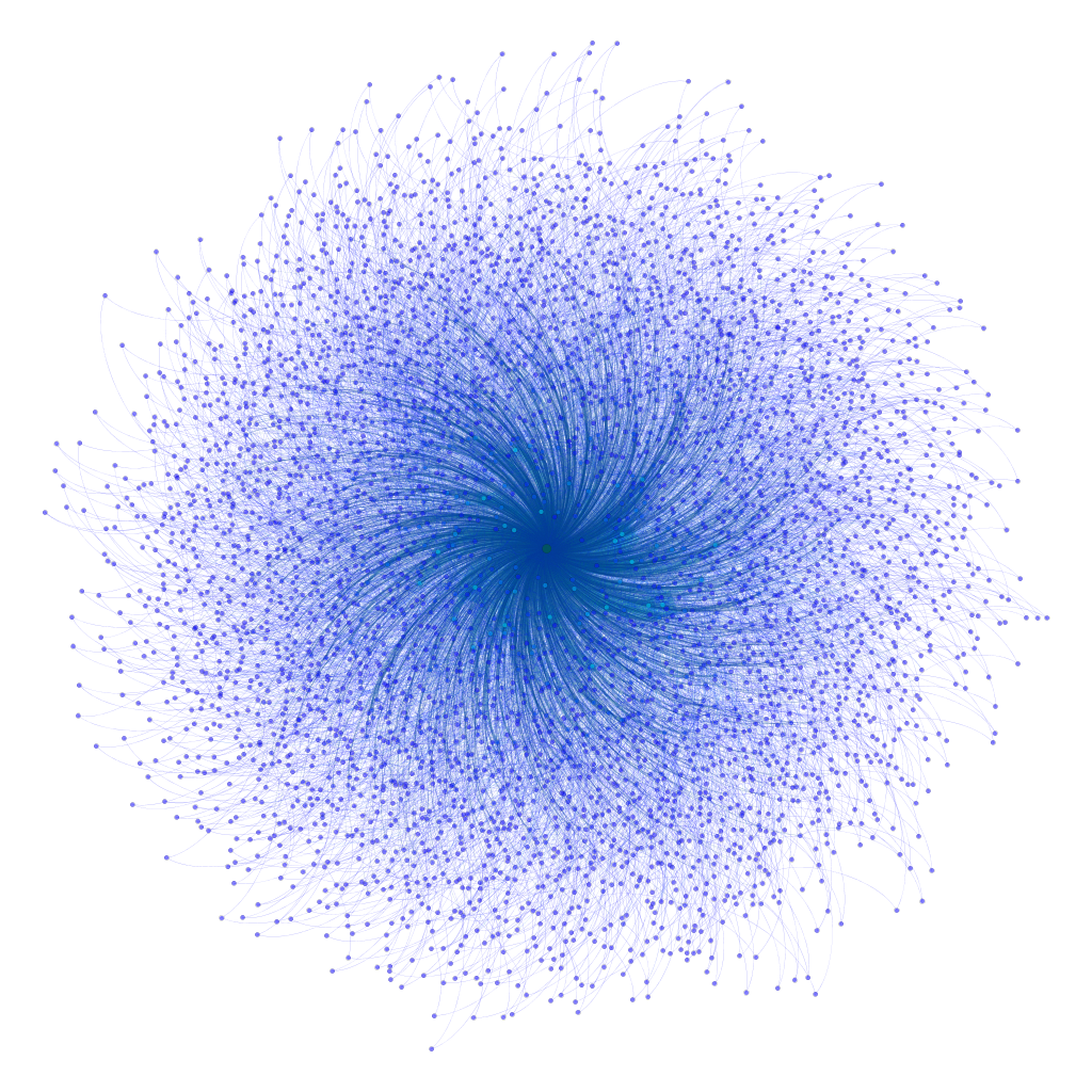
Computing the number of triangles $\blacktriangle$ becomes simple, once you know the eigenvalues.

$\blacktriangle = \frac{1}{6} \sum\limits_{i = 1}^{N} \lambda_i^3$

Network spectra

Random network

Barbasi-Albert ($N$ = 5000)
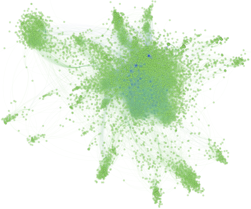
a sample network a sample network

Network of AS

tech-WHOIS, Mahadevan, P., Krioukov, D. et al. ($N$ = 7476)

a sample network a sample network

The adjacency and the Laplacian spectra might not be as intuitive for humans as the graph representation, but both contain the complete information about the topology of the network.

Can we extract the hidden relations between the properties of a network and their corresponding spectra?

Proof of concept: counting triangles

  • Idea: use Cartesian Genetic Programming (CGP) to evolve symbolic expression!
    1. generate all networks with $N = 6$ nodes
    2. compute $\blacktriangle$ as target
    3. compute $\lambda_1, \ldots, \lambda_6$ as features
  • Does it work?
    1. allow operations $\{+,\cdot^3\}$, do not bother with the constant $\frac{1}{6}$
    2. $6\blacktriangle = \sum\limits_{i = 1}^{6} \lambda_i^3$ in 99%!Okay, that was too easy...
    3. allow operations $\{+,\times,\cdot^3\}$, give constant $\frac{1}{6}$ as input node
    4. $\blacktriangle = \frac{1}{6}\sum\limits_{i = 1}^{6} \lambda_i^3$ in 15%!Probably still expected?
    5. allow operations $\{+,\times,\div,\cdot^3\}$, only constants $\{1,2,3\}$ as input nodes
    6. $\blacktriangle = \frac{1}{6}\sum\limits_{i = 1}^{6} \lambda_i^3$ in 2%!Maybe this could really work!?

Rediscover a known formula for a network property

Discover an unknown formula for a network property

Network diameter

Length of the longest of all shortest paths in a network.


								def diameter(G):
								    diam = 0
								    for src, dest in zip(G.nodes(), G.nodes()):
								        path = shortest_path(src, dest)
								        diam = max(len(path), diam)
								    return diam
							

The exact formula for the network diameter $\rho$ implies this exhaustive enumeration:

$$\rho = \max\limits_{src, dest} \min dist(src, dest)$$

a sample network

In this example the diameter is 3.

Why are we interested in the diameter anyway?

Diameter = worst-case lower bound on number of hops
i.e. limits the speed of spreading/flooding in a network

Symbolic regression for the diameter

  • Idea: Try (systematically) different configurations with CGP!
    1. generate all networks with $N = 6$ nodes
    2. compute $\rho$ as the target
    3. compute $\lambda_1, \ldots, \lambda_6$ as features
    4. include $N, L$ and some basic constants $\{1,2,3\}$ as features as well
    5. use different sets of operators like $\{+,-,\times,\cdot^2\}$ or $\{+,-,\times,\div,\sqrt{\cdot}\}$

Pick the expression that minimizes the sum of absolute errors:

$f(\hat{\rho}) = \sum\limits_{G} \mid \rho(G) - \widehat{\rho(G)} \mid$

  • Does it work?
  • $\hat{\rho} = 2$What happened?

Target distributions

Triangles $\blacktriangle$

Diameter $\rho$

Exhaustive learning on all networks is no longer feasible.

Networks need to be sampled to create a good (diverse) learning set.

Sampling networks

Augmented path graphs

aug path $\rho = 11$
aug path $\rho = 10$
aug path $\rho = 8$
  • sparse networks
  • varies $\rho$ by keeping $N$ constant

Barbell graphs

aug path $\rho = 6$
aug path $\rho = 8$
aug path $\rho = 8$
  • dense networks
  • varies $N$ by keeping $\rho$ constant

Mixed graphs

50% augmented path + 50% barbell

Computation pipeline

computation pipeline

CGP parametrization

parameter value
fitness function sum of absolute errors
evolutionary strategy 1+4
mutation type and rate probabilistic (0.1)
node layout 1 row
200 columns
levels-back unrestricted
number of generations 200000
operators $+,-,\times,\div,\cdot^2,\cdot^3,\sqrt{\cdot},\log$
constants $1,2,3,4,5,6,7,8,9$
featuresets A) $N,L,\lambda_1,\lambda_2,\lambda_3,\lambda_N$
B) $N,L,\mu_1,\mu_{N-1},\mu_{N-2},\mu_{N-3}$

Automatically generated formulas

$\begin{equation} \hat{\rho} = \frac{\log{\left (2 L \mu_{N-3} + 6 \right )} + 6}{\log{\left (L \mu_{N-3} + \sqrt{5} \sqrt{\frac{1}{\mu_{N-1}}} \right )}} + \sqrt{5} \sqrt{\frac{1}{\mu_{N-1}}} + 3 \sqrt{82} \sqrt{\frac{1}{729 L \mu_{N-2} \mu_{N-3} - 5}} \end{equation}$

$\begin{equation} \hat{\rho} = N - \frac{1 - \frac{1}{\left(L - N\right)^{\frac{3}{2}}}}{\frac{6 - \frac{6}{\left(L - N\right)^{\frac{3}{2}}}}{\sqrt{L - N}} + 4 \sqrt{L - N}} - 2 \sqrt{L - N} - \frac{1}{\sqrt{L - N}} \end{equation}$

$\begin{equation} \hat{\rho} = \sqrt{\sqrt{N} + \frac{45 \mu_{N-3}}{\left(\mu_{N-1} + \mu_{N-3}\right)^{2}} + \log{\left (\frac{216}{\left(\mu_{N-1} + \mu_{N-3}\right)^{2}} \right )} - \frac{16}{9 \mu_{N-3}} + \frac{8 \sqrt[4]{\mu_{N-3}}}{L \mu_{N-1} \mu_{N-2}}} \end{equation}$

Bounds on the diameter

$\begin{equation} \hat{\rho} = \frac{\log{\left (2 L \mu_{N-3} + 6 \right )} + 6}{\log{\left (L \mu_{N-3} + \sqrt{5} \sqrt{\frac{1}{\mu_{N-1}}} \right )}} + \sqrt{5} \sqrt{\frac{1}{\mu_{N-1}}} + 3 \sqrt{82} \sqrt{\frac{1}{729 L \mu_{N-2} \mu_{N-3} - 5}} \end{equation}$

Comparison to known analytical results from graph theory:

Upper bound by Chung, F.R., Faber, V. and Manteuffel, T.A.: "An Upper bound on the diameter of a graph from eigenvalues associated with its Laplacian."

(See also Van Dam, E.R., Haemers, W.H.: "Eigenvalues and the diameter of graphs.")

$\rho \leq \left\lfloor \frac{\cosh^{-1}(N-1)}{\cosh^{-1}\left(\frac{\mu_1 + \mu_{N-1}}{\mu_1 - \mu_{N-1}}\right)}\right\rfloor + 1$

$\hat{\rho}/\rho$

This is how it looks

Diameter on real networks

parameter value
$N$ 379
$L$ 914
true diameter $\rho$ 17
approximated diameter $\hat{\rho}$ 21.48
upper bound 160.09
ca-netscience

ca-netscience ca-netscience

source: http://www.networkrepository.com

Diameter on real networks

parameter value
$N$ 4941
$L$ 6594
true diameter $\rho$ 46
approximated diameter $\hat{\rho}$ 97.52
upper bound 749.49
ca-netscience

Diameter on real networks

parameter value
$N$ 1458
$L$ 1948
true diameter $\rho$ 19
approximated diameter $\hat{\rho}$ 18.59
upper bound 207.52
bio-yeast network

Diameter on real networks

Diameterplot overview

Can we extract the hidden relations between the properties of a network and their corresponding spectra?

Closing thoughts

  • Automatically evolving approximate equations for network properties is possible.
  • Equations are unbiased by human preconceptions.
  • Unexpected results may aid and stimulate research in spectral graph theory and network science in general.

Challenges and possible (?) improvements

  • Sampling network space for stronger diversity.
  • Make complexity of formula part of the objective function.
  • Automatically evolve constants rather than using them as inputs.
  • Apply more advanced feature-selection methods to increase quality of formulas.