A Time-dependent SIS-model for Long-term Computer Worm Evolution
Marcus Märtens, Hadi Asghari, Michel van Eeten and Piet Van Mieghem


“In theory, there is no difference between theory and practice. But, in practice, there is.”Jan L. A. van de Snepscheut
Scientific modelling

Data from Conficker Worm
population-based SIR-Model
Infected
Removed

Changing assumptions
- fixed population of N individuals
- mutual contact between all individuals
- number of susceptible hosts are monotonously decreasing
- constant infection rate $\beta$
- constant curing rate $\delta$
Towards a more general model
- mutual contact between all individuals
- $r$-regular contact network
- number of susceptible hosts are monotonously decreasing
- reinfection enabled by SIS instead of SIR
- constant infection rates and curing rates
- time-dependent infection and curing rates $\beta(t), \delta(t)$
What do we want to know?
How does the prevalence of a computer worm evolve over time?
$\Downarrow$
$y(t)$: average fraction of infected nodes at time $t$
NIMFA closed form for $r$-regular networks
$\frac{dy(t)}{dt} = \beta r y(t) (1 - y(t)) - \delta y(t)$
$\Downarrow$
$y(t) = \frac{y_0y_{\infty}}{y_0 + (y_{\infty} - y_0) e^{-(\beta r - \delta)t}}$
- $r$: degree of every node in network
- $y(t)$: average fraction of infected nodes at time $t$
- $y_0(t)$: initial fraction of infected nodes
- $y_\infty$: steady-state fraction of infected nodes
time-dependent NIMFA
$\frac{dy(t)}{dt} = \color{red}{\beta(t)} r y(t) (1 - y(t)) - \color{blue}{\delta(t)} y(t)$
has as solution
$y(t) = \frac{e^{\color{green}{\rho(t)}}}{\frac{1}{y_0} + r \int_0^t \color{red}{\beta(s)} e^{\color{green}{\rho(s)}} ds}$
with
$\color{green}{\rho(t)} = \int\limits_{0}^{t}(r\color{red}{\beta(u)} - \color{blue}{\delta(u)}) du$
- $\beta$ and $\delta$ can now change with time!
Conficker

- First detected November 2008
- Sinkholed February 2009
- 9M infected machines world-wide at highest peak
- Worm remained active for years (difficult cleanup)
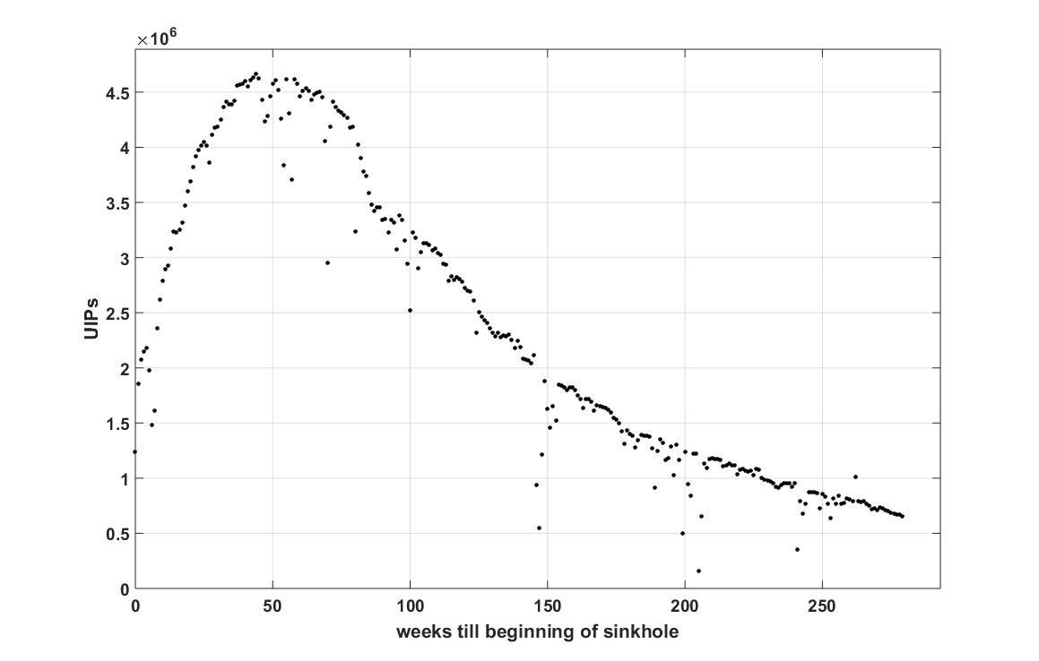
Data pre-processing
Raw data: sinkhole logfiles
- Botnet size estimation: UIPs vs machines
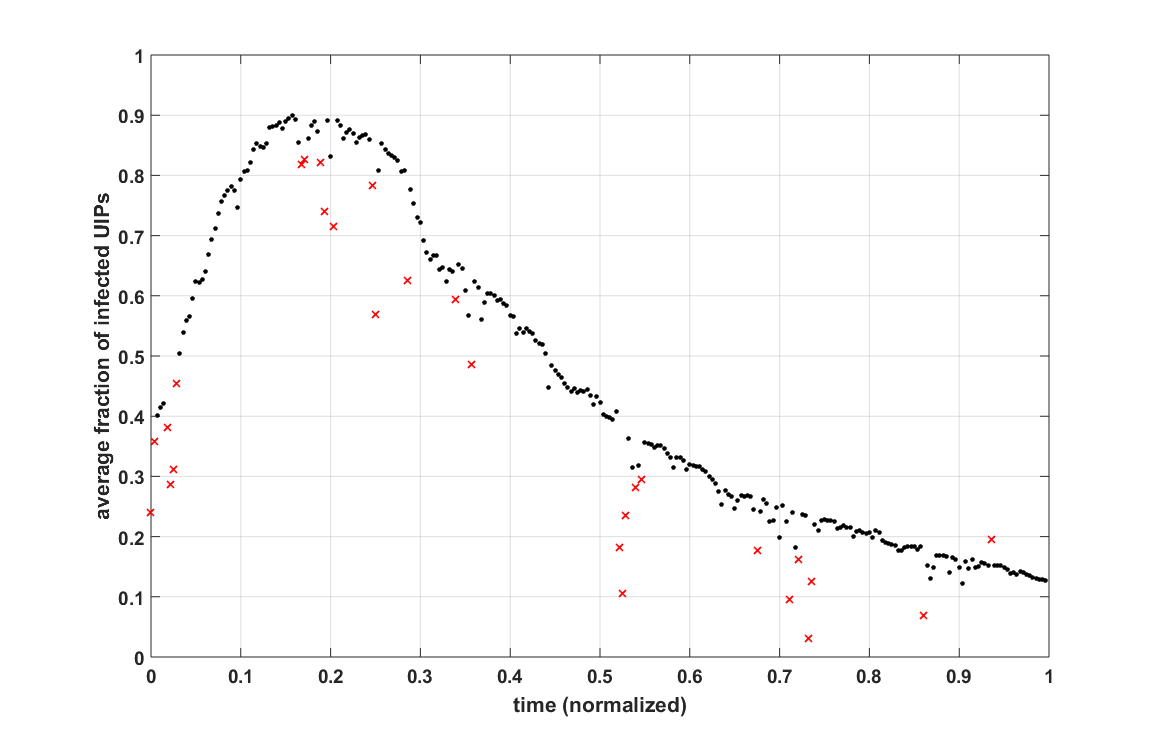
- Data cleansing: removing outliers
- Normalization: scaling factor $s_y$
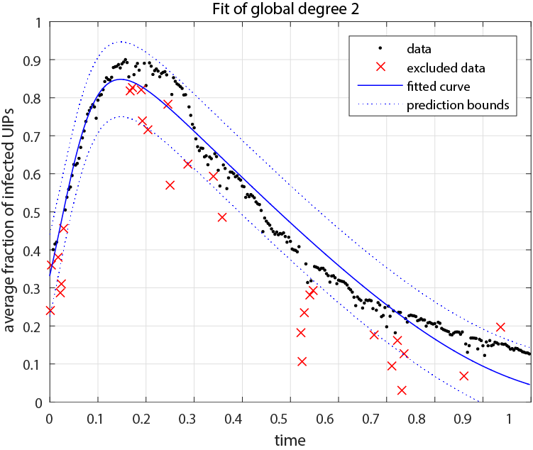
Conficker: Global level
Results: Candidate models
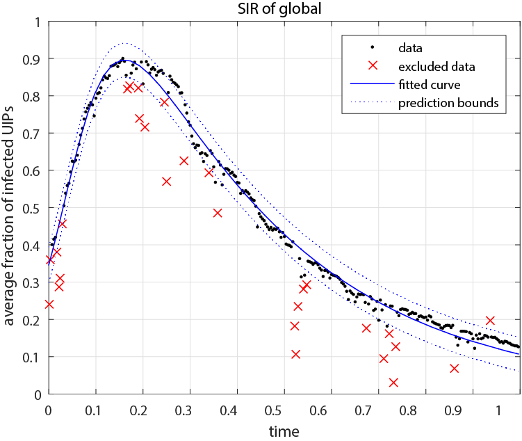
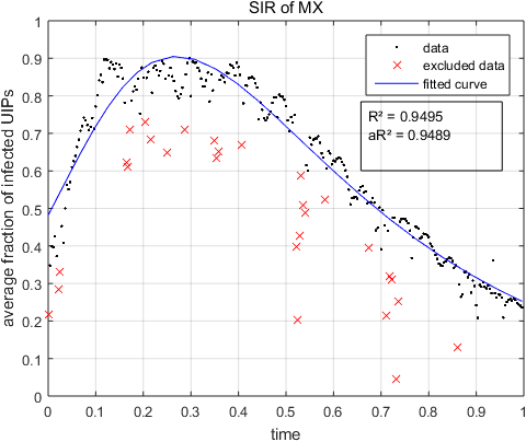
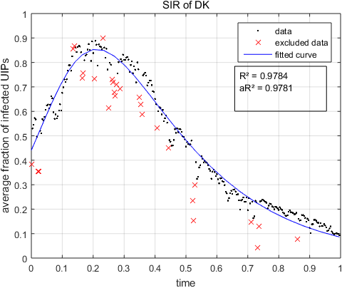
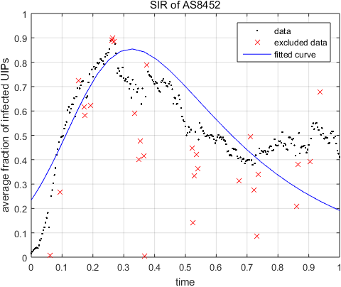
- The baseline: SIR
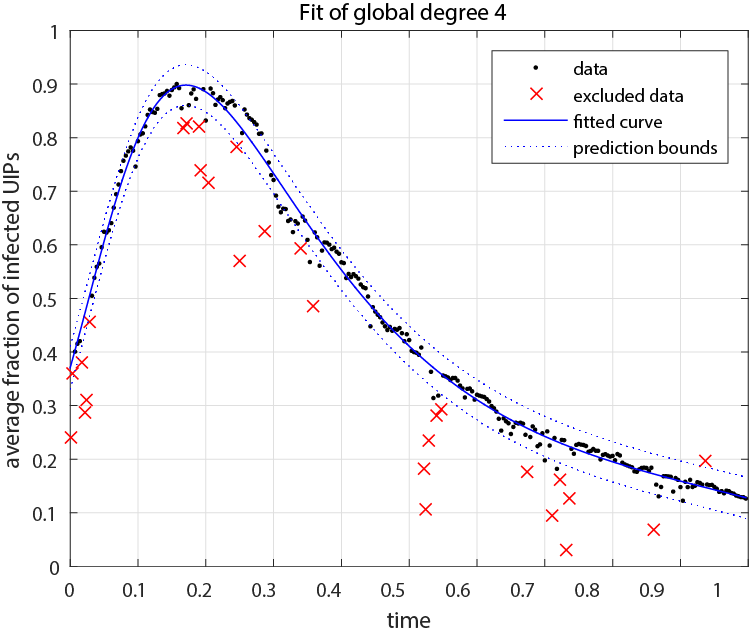
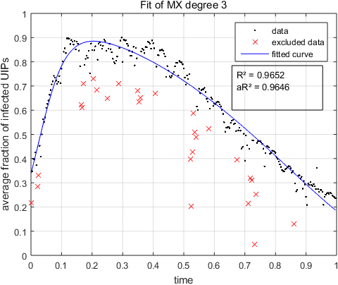
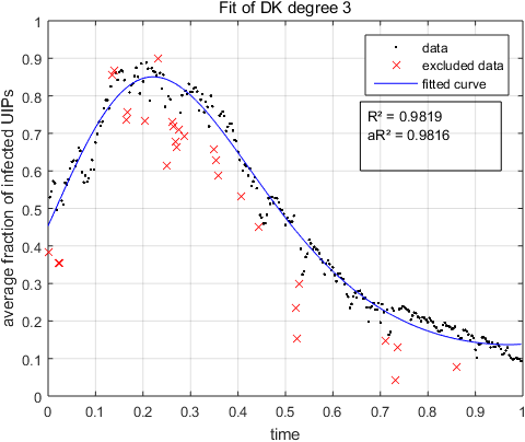
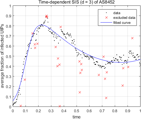
- The challenger: time-dependent NIMFA (TD-SIS)
- Assumption: worm spreading pattern did not change over time
- Assumption: clean-up effort increases after discovery
- Assumption: clean-up effort saturates if all counter-measures are deployed
Taylor-expansion to approximate $D(t)$ yields a polynomial for $\delta(t)$ with degree $d$
Results: Global Level


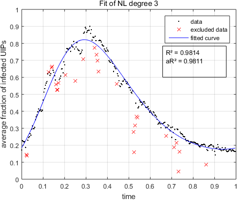
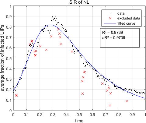
Results: Country Level
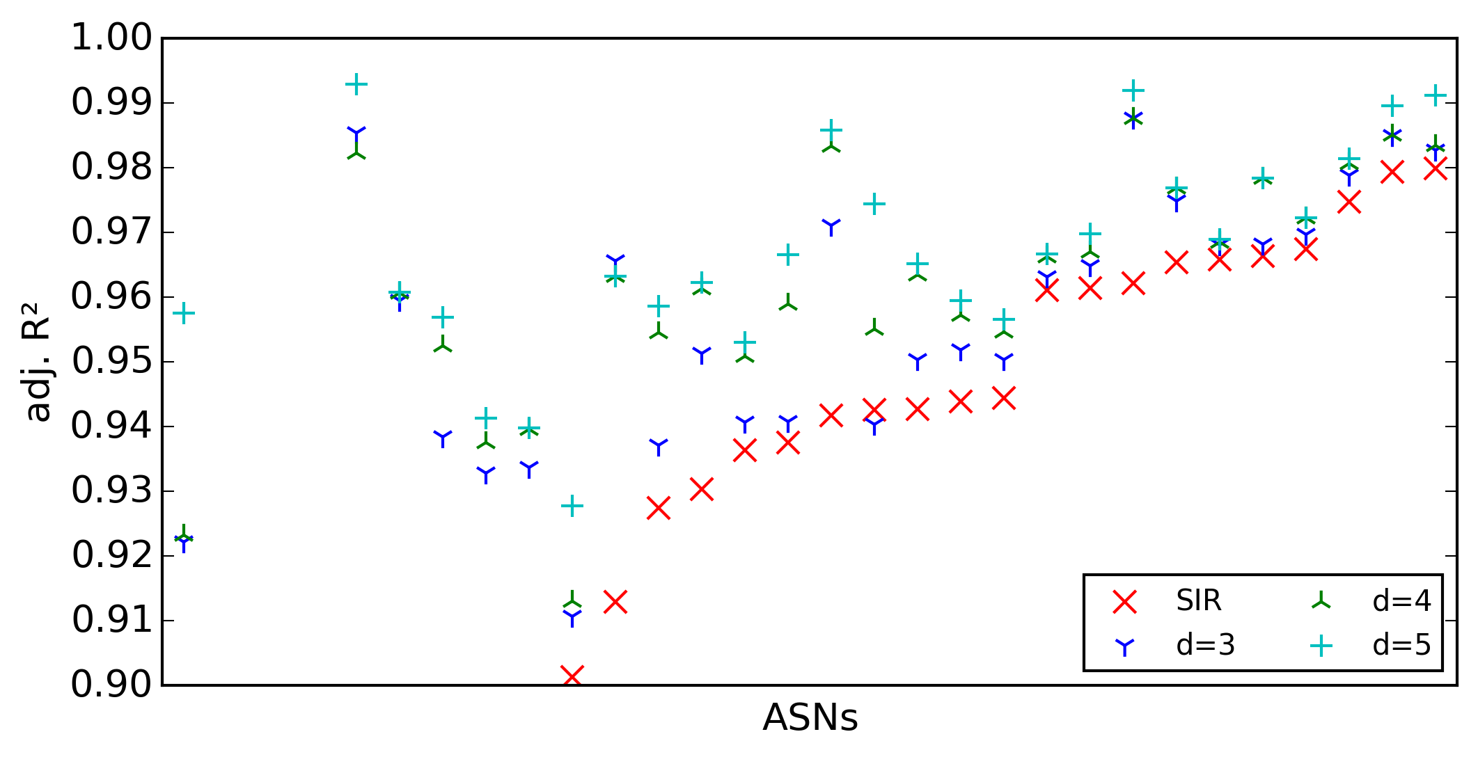
Results: ASN Level
Curing-rate function (global scale)
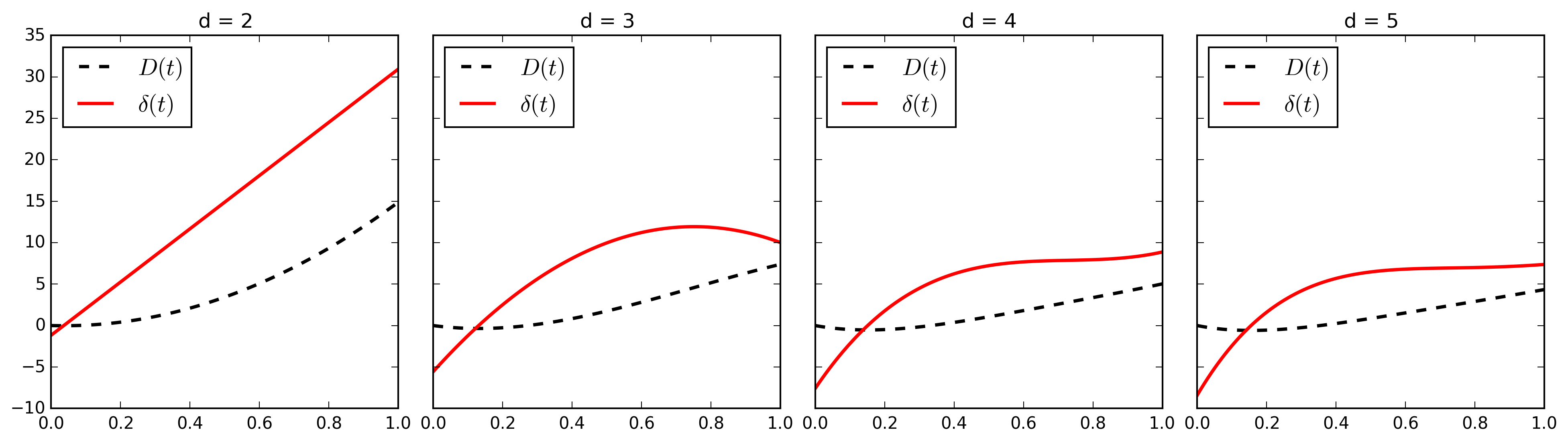
saturation behavior for higher order approximation
Conclusions
- TD-SIS is able to describe the following effects
- reinfection
- altering worm spreading power
- increasing/decreasing counter-measures
- SIR limited to monotone spreading and decline
- Measurement of model parameters could lead to a potential monitoring system
Additional material
(Backup slides)
Intermediaray epidemic models
population-based SIS-Model
Infected
Susceptible
- fixed population of $N$ individuals
- mutual contact between all individuals
- reinfection possible (non-monotonous)
- constant infection rate $\beta$
- constant curing rate $\delta$
network-based mean-field SIS-Model (NIMFA)
$\frac{dv_i(t)}{dt} = -\delta v_i(t) + \beta(1 - v_i(t))\sum\limits_{j = 1}^{N} a_{ij}v_j(t)$- $v_i(t)$: probability of node $i$ to be infected at time $t$
- $A = (a_{ij})$: adjacency matrix of network
- reinfection possible (non-monotonous)
- constant infection rate $\beta$
- constant curing rate $\delta$
NIMFA for $r$-regular networks
$\frac{dv_i(t)}{dt} = -\delta v_i(t) + \beta(1 - v_i(t))\sum\limits_{j = 1}^{N} a_{ij}v_j(t)$
$\Downarrow$ by symmetry $v_i(t) = v(t) = y(t)$
$\frac{dy(t)}{dt} = \beta r y(t) (1 - y(t)) - \delta y(t)$
- $r$: degree of every node in network
- $v_i(t)$: probability of node $i$ to be infected at time $t$
- $y(t)$: average fraction of infected nodes at time $t$
- $y_0(t)$: initial fraction of infected nodes
- $y_\infty$: steady-state fraction of infected nodes
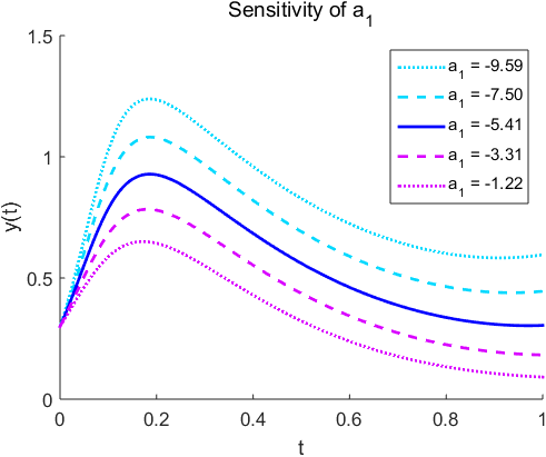
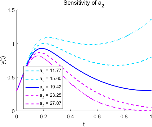
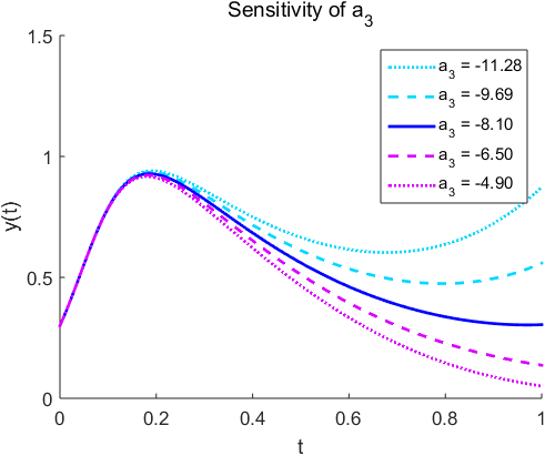
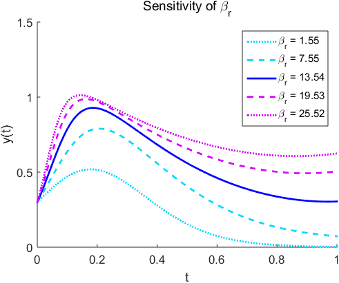
Sensitivity
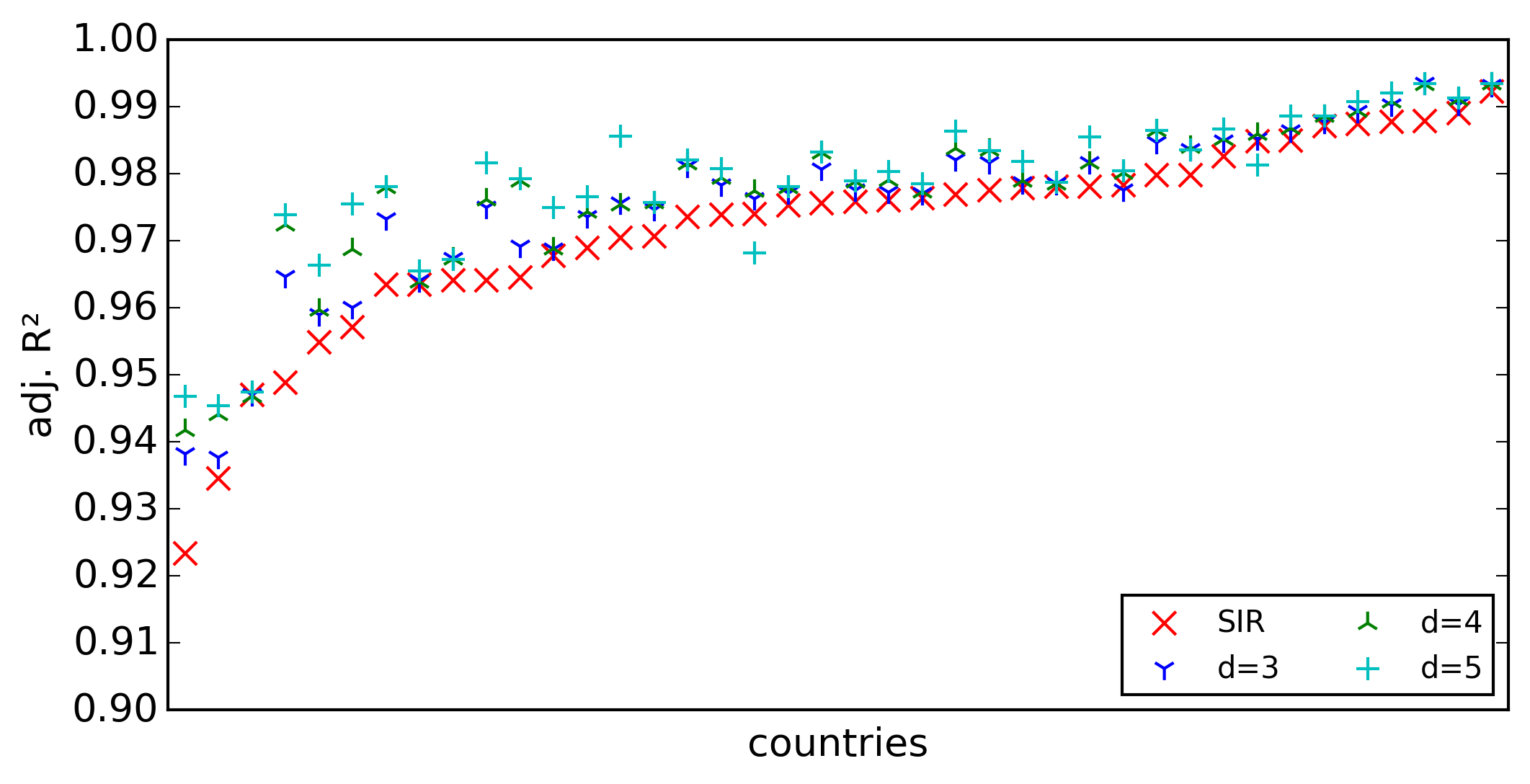
Quality of fit
Country-level
ASN-level